Chart nonconformities per exposure

Chart nonconformities per exposure

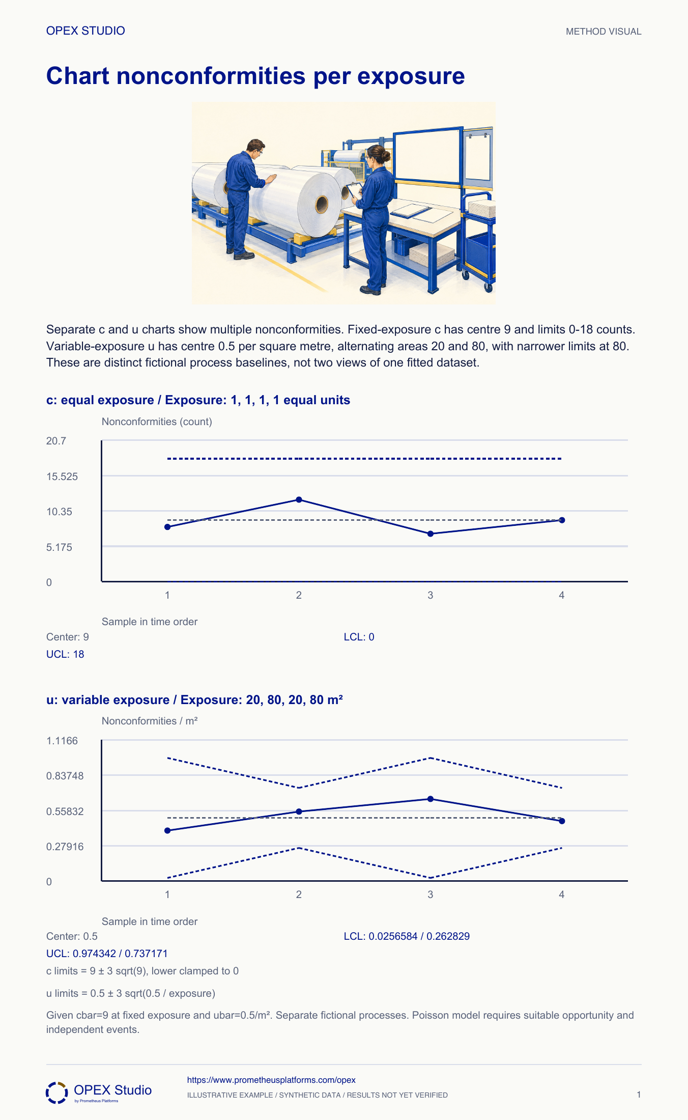
A nonconformity count is not restricted to one per product. A c chart is a basic candidate when inspection exposure and opportunity are comparable. A u chart expresses nonconformities per unit of exposure when the amount inspected varies. Keep the original count and exposure with every point so the displayed rate can be checked. The basic formulas rely on a suitable count model; clustering, changing opportunity and very low expected counts can invalidate a casual interpretation. Do not compare rates from incompatible definitions of area, time or opportunity. The two panels here describe separate fictional baselines and should not be combined into one process.

Follow the method

1. c: equal exposure
2. Nonconformities (count)
3. Sample in time order
4. Center: 9
5. LCL: 0
6. UCL: 18
7. u: variable exposure
8. Nonconformities / m²
9. Center: 0.5
10. LCL: 0.0256584 / 0.262829
11. UCL: 0.974342 / 0.737171

Preserve the opportunity behind every nonconformity rate

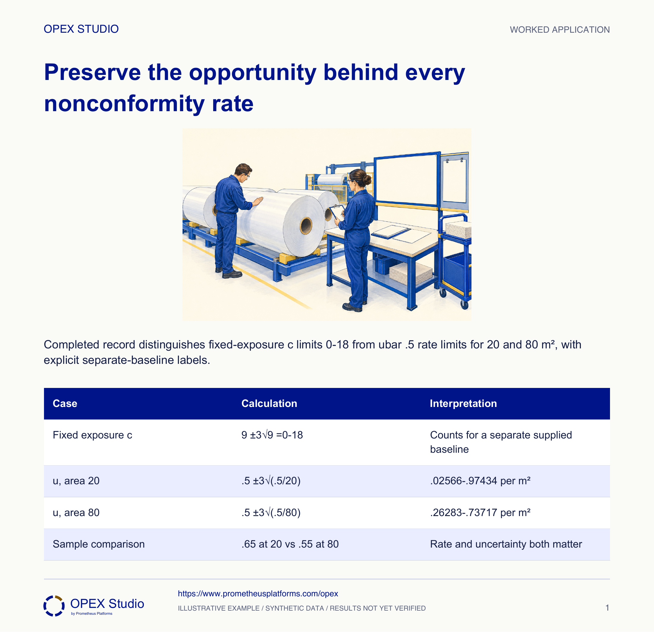
Fictional case: a surface-inspection team counts blemishes, with several possible on one sheet. The core c chart is a separate fixed-exposure process with supplied cbar 9 and counts 8,12,7,9. The u example has supplied ubar .5 per square metre, areas 20,80,20,80 and counts 8,44,13,38. Analyst Hugo must keep the two baselines and scales separate.

Follow the method

1. Fixed exposure c
2. u, area 20
3. u, area 80
4. Sample comparison

A larger inspected area offers more opportunities

Distinguish counts of multiple nonconformities from affected-unit fractions and account for the actual opportunity exposed to inspection.

Fictional case: a surface-inspection team counts blemishes, with several possible on one sheet. The core c chart is a separate fixed-exposure process with supplied cbar 9 and counts 8,12,7,9. The u example has supplied ubar .5 per square metre, areas 20,80,20,80 and counts 8,44,13,38. Analyst Hugo must keep the two baselines and scales separate.

Role: Surface-quality analyst and inspection lead

Normal condition

The record defines a blemish, the inspected opportunity and comparable conditions. Counts and exposure remain available, even when rates are displayed.

The gap

The team calls 44 blemishes worse than 13 without considering 80 versus 20 square metres, and combines both fictional baselines into one calculation.

• The two core panels are separate illustrative processes, not a common fitted dataset.
• A suitable count model and comparable opportunity are assumptions to check; clustering or skewed rare counts need care.

1. Define the event and opportunity

   Hugo specifies a blemish category and square metres actually examined under the same inspection definition. He distinguishes these multiple events from a pass/fail classification of each sheet.

   Why: A sheet may contain several events. A p chart of affected sheets would answer a different question from blemishes per area.

   Evidence: The collection record contains count, actual area and inspection context.

2. Use c only for its fixed comparable exposure

   For the separate fixed-exposure example, limits are 9 ±3√9, or 0 and 18 counts. He retains cbar 9 as the supplied historical baseline.

   Why: A count comparison assumes the opportunity is comparable. Applying it to a much larger inspected area could produce a signal caused merely by exposure.

   Evidence: The c panel is labelled counts at fixed exposure, with no borrowed u baseline.

3. Calculate the u rates

   Hugo divides count by area:8/20=.40,44/80=.55,13/20=.65 and 38/80=.475 per m². He checks each numerator against its inspection record.

   Why: The largest count is not necessarily the largest rate. Area units must remain consistent; square centimetres cannot silently be used in a per-square-metre calculation.

   Evidence: Four point-specific rates retain their actual areas.

4. Apply exposure-specific uncertainty

   For ubar .5, limits are .5 ±3√(.5/area). Area 20 gives approximately .02566–.97434; area 80 gives .26283–.73717 per m².

   Why: Larger exposure narrows the rate limits under the assumed count model. The center remains the supplied rate; the changing limits are not product specifications.

   Evidence: The native record displays the correct limits beside each observation.

5. Qualify the interpretation and response

   Hugo checks whether blemishes cluster or opportunities differ by product/area. He records signals and asks the owner to review the model if those conditions undermine it.

   Why: A computed limit is not proof that the count model fits. A response should preserve the event and exposure records and use authorized product/operating decisions.

   Evidence: The investigation separates model adequacy, signal evidence and disposition authority.

Inspection includes a different surface type

An 80 m² observation combines a smooth coating with a textured surface having different inspection difficulty and opportunity.

Preserve the record and review stratification and opportunity definitions before treating the combined area as comparable exposure.

A numerical area alone may not represent equivalent opportunity. A larger denominator can conceal a collection or process mixture.

The revised collection plan identifies surface type and comparable exposure.

Run a practice session

Materials

• Area/count cards
• Calculator
• Two separately titled process records

1. Define a blemish event · 5 minutes

   How can one sheet contribute several?

2. Compare rate and count · 8 minutes

   Why is 44 not automatically worse than 13?

3. Work the changed observations · 10 minutes

   Which baseline belongs to each?

4. Debrief opportunity · 5 minutes

   When does equal area fail to mean equal opportunity?

Debrief

• Ask for per-m² units on the u calculation.
• Keep the c and u examples physically separate during the exercise.

Calculate each rate from its own count and area before examining limits.

Transfer into the work

Owner: Inspection-method and SPC owners

Record: Event/exposure record, model rationale and reaction log

Review: At each observation and after surface or inspection changes

Evidence: Comparable opportunity, traceable counts and appropriate response

Revisit sampling or model choice if clustering, exposure or classification changes invalidate the comparison.