Facilitator guide
Case objectives, demonstration plans, debriefs, common mistakes and application checks across all 81 workplace cases and method lessons.
Download Facilitator guide PDF · 166 pages · 65.1 MB OPEXSTUDIO
Define available time and demand. Follow the visual, practise a decision, then check your thinking.
Fictional teaching examples and AI-generated illustrations. Proposed changes and goals are not achieved results. Use the written instructions and check local conditions before applying a method.
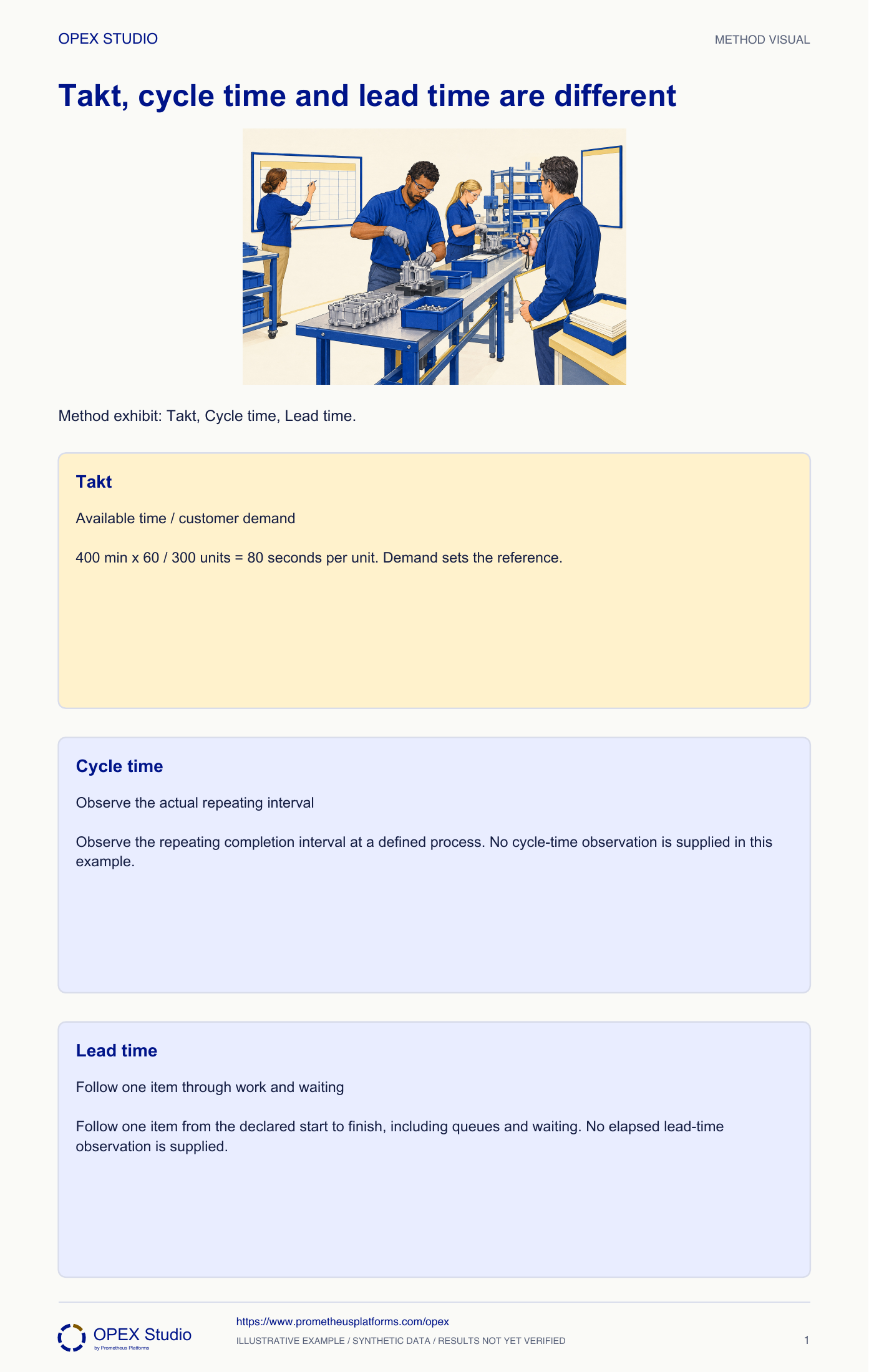
Use three clocks to avoid three different questions becoming one number. Takt expresses the demand interval over a declared available period. Cycle observations describe how a process actually repeats, including its variation. Lead time follows one order through work and waiting from an agreed beginning to an agreed end. In this exercise, 400 available minutes for 300 units gives an 80-second takt. That is a planning reference, not proof that every task can safely be performed in 80 seconds. Investigate gaps in method or capacity and verify the effect on customer elapsed time.
Takt = 400 available min × 60 / 300 units = 80 sec/unit for this fictional horizon.
Cycle time requires actual process observations; lead time follows an item through both work and waiting. Neither is supplied as a measured result here.
Changing the time boundary or product mix changes the meaning of the comparison. Keep units and assumptions explicit.
Fictional assembly planning case: a team has 400 net available minutes and demand for 300 units. Supervisor Bea is asked whether the line is fast enough and whether a customer order can be promised tomorrow. The supplied concept gives no measured cycle time or order lead time.
Use 450 minus 50 = 400 net minutes; the takt stays 80 seconds per unit.
Dividing gross time would give 90 seconds and imply more productive time than the plan provides.
Calculate takt from net time and demand, distinguish it from observed cycle and lead time, and label missing measurements instead of inventing performance.
Fictional assembly planning case: a team has 400 net available minutes and demand for 300 units. Supervisor Bea is asked whether the line is fast enough and whether a customer order can be promised tomorrow. The supplied concept gives no measured cycle time or order lead time.
Role: Assembly supervisor with the planner and an operator observer.
Time measures carry a defined start, finish, unit and operating condition before they are compared.
A planning sheet copies the demand-derived 80 seconds into the actual cycle and order lead-time boxes.
| Measure / input | Supplied value or boundary |
|---|---|
| Net available time | 400 min per planning day |
| Customer demand | 300 units in that day |
| Takt | To calculate; sec per required unit |
| Observed cycle | Not supplied; specify repeat-event boundary |
| Order lead time | Not supplied; specify receipt and completion boundary |
Bea checks that the 400 minutes and 300 required units refer to the same planning period and product mix. She converts minutes to seconds before dividing.
Why: Mismatched periods or gross versus net time create a demand rhythm that looks precise but answers the wrong question.
Evidence: 400 × 60 = 24,000 available seconds.
Divide 24,000 seconds by 300 units and label the result 80 seconds per required unit. Keep it in the planning reference column.
Why: Takt comes from available time and demand. It is not a measurement of how long an operator or order actually took.
Evidence: Takt = 80 sec/unit; demand basis and planning day recorded.
Agree a repeatable process event, such as successive completion of the same assembly operation, and plan repeated observations across relevant conditions. Record abnormal events and mix rather than silently discarding them.
Why: A repeatable boundary makes observed cycle data interpretable. A single selected fast cycle cannot establish reliable capacity.
Evidence: Cycle-time field remains “not measured”; observation boundary and conditions are named.
Trace an identified order from accepted receipt to verified completion, stating whether the unit is working hours or elapsed calendar hours. Include waiting inside that chosen boundary.
Why: Lead time spans the route and can be far longer than the time spent processing. An 80-second takt cannot support a next-day promise.
Evidence: Order start/finish timestamps and boundary are still required.
Publish the 80-second demand reference and a measurement plan. Defer claims of achieved rate or delivery promise until cycle variation, route delays and capacity conditions are available.
Why: Separating a known calculation from unknown observations prevents a target from being reported as a result.
Evidence: Three named fields: calculated takt, measured cycle, measured order lead time.
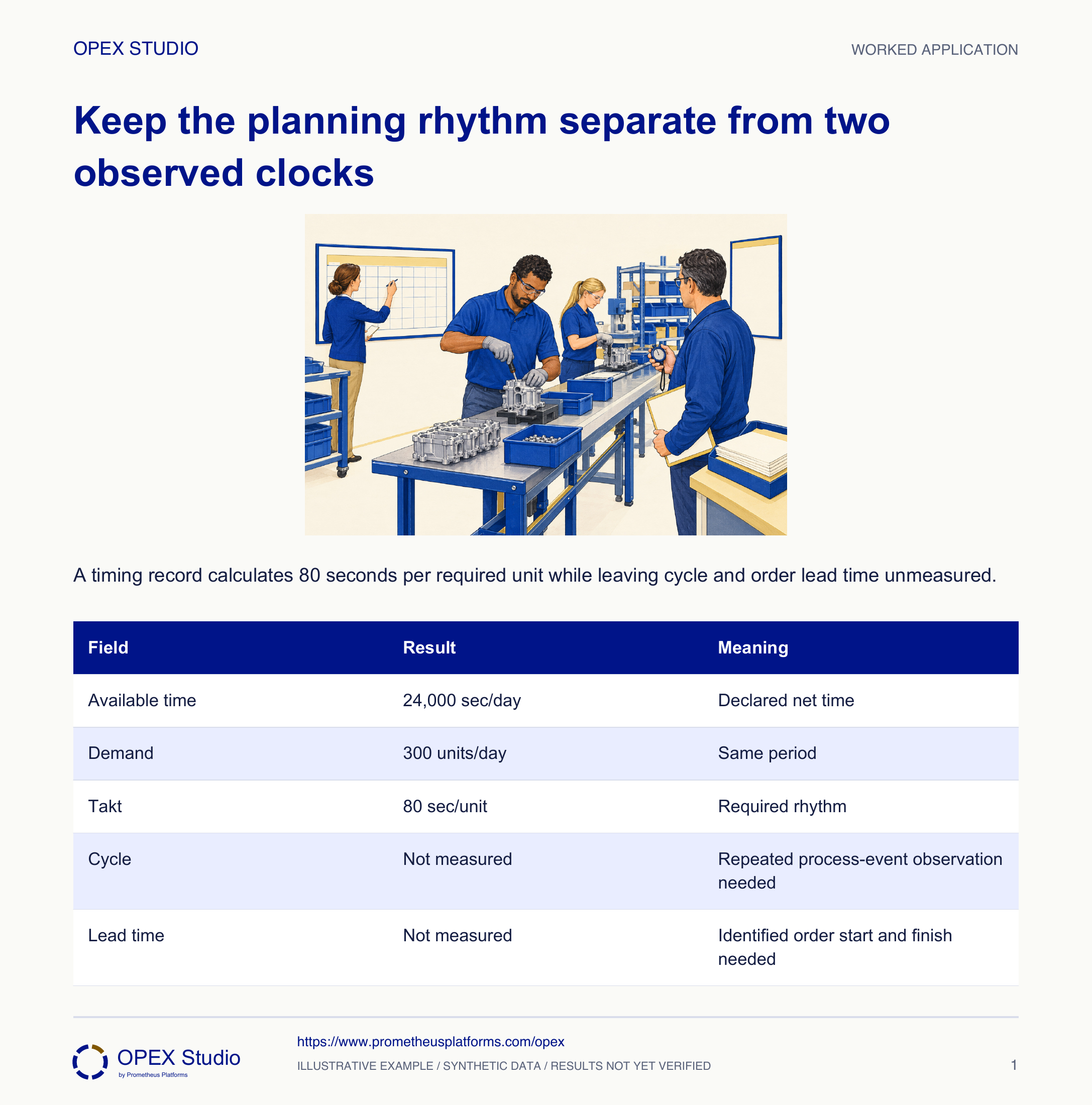
| Field | Result | Meaning |
|---|---|---|
| Available time | 24,000 sec/day | Declared net time |
| Demand | 300 units/day | Same period |
| Takt | 80 sec/unit | Required rhythm |
| Cycle | Not measured | Repeated process-event observation needed |
| Lead time | Not measured | Identified order start and finish needed |
Another planner supplies 450 minutes including 50 minutes of planned nonproduction time for the same 300 units.
Use 450 minus 50 = 400 net minutes; the takt stays 80 seconds per unit.
Dividing gross time would give 90 seconds and imply more productive time than the plan provides.
Both versions reconcile to 24,000 net seconds.
Separate fictional case: 360 net minutes, 240 required units; five observed process intervals are 82, 88, 94, 86 and 90 seconds. Order K is accepted Monday at 09:00 and completes Tuesday at 15:00. Use elapsed calendar hours.
| Input | Value |
|---|---|
| Net time / demand | 360 min / 240 units |
| Observed intervals | 82, 88, 94, 86, 90 sec |
| Order K start | Monday 09:00 |
| Order K finish | Tuesday 15:00 |
Takt is 360 × 60 / 240 = 90 sec/unit. The five observed intervals total 440 seconds, so their mean is 88 seconds.
Order K spans 30 elapsed calendar hours. That does not mean 30 hours of touch work.
One observed interval is 94 seconds, above takt, and five intervals are not a sufficient capability study. State the sample and investigate variation, losses and mix before promising performance.
| Measure | Calculation / evidence | Result |
|---|---|---|
| Takt | 21,600 / 240 | 90 sec/unit |
| Sample mean | 440 / 5 | 88 sec |
| Observed range | 82 to 94 | One interval exceeds takt |
| Lead time | 24 plus 6 | 30 calendar hours |
Which value can be calculated from the supplied original inputs?
Why must two boxes remain unmeasured?
Does 88 below 90 settle the capacity question?
Which event boundaries and conditions will you record?
Calculate independently, then explain each result as one sentence containing its unit and boundary.
Owner: Process owner with planning and trained observers
Record: Demand/net-time basis, repeated cycle sheet and order timestamp trace
Review: When demand or time basis changes, and after the agreed observation period
Evidence: Traceable definitions, representative observations and a decision consistent with variation
Keep capacity and promise claims provisional; obtain missing timing and route evidence.
Demand-paced available production time per required unit.
Method reference; original OPEX scenario and diagram are synthetic teaching content, not source case results.Read the lessons online or use these PDFs to prepare, practise and review with your team. No sign-in needed.
Case objectives, demonstration plans, debriefs, common mistakes and application checks across all 81 workplace cases and method lessons.
Download Facilitator guide PDF · 166 pages · 65.1 MBPrintable case worksheets, blank observation records and five calculation exercises; answers are separate.
Download Learner workbook PDF · 169 pages · 10.7 MBReasoned sample responses, worked calculations and coaching guidance; fictional examples are clearly labelled.
Download Answer key and coaching notes PDF · 105 pages · 8.5 MBThe native method mechanisms and worked applications for all 68 detailed lessons, in a separate bookmarked portrait reference.
Download Method and application reference PDF · 141 pages · 10.2 MBFive illustrated system chapters: 15 Flare concept maps and 26 original workplace teaching cards, with links to all 81 supporting cases and method lessons.
Download Illustrated systems atlas PDF · 69 pages · 55.8 MBExplore this connected method and its separate application conditions.
Explore the connected method →Explore this connected method and its separate application conditions.
Explore the connected method →Explore this connected method and its separate application conditions.
Explore the connected method →Explore this connected method and its separate application conditions.
Explore the connected method →