Facilitator guide
Case objectives, demonstration plans, debriefs, common mistakes and application checks across all 81 workplace cases and method lessons.
Download Facilitator guide PDF · 166 pages · 65.1 MB OPEXSTUDIO
Define the measured characteristic and unit.. Follow the visual, practise a decision, then check your thinking.
Fictional teaching examples and AI-generated illustrations. Proposed changes and goals are not achieved results. Use the written instructions and check local conditions before applying a method.
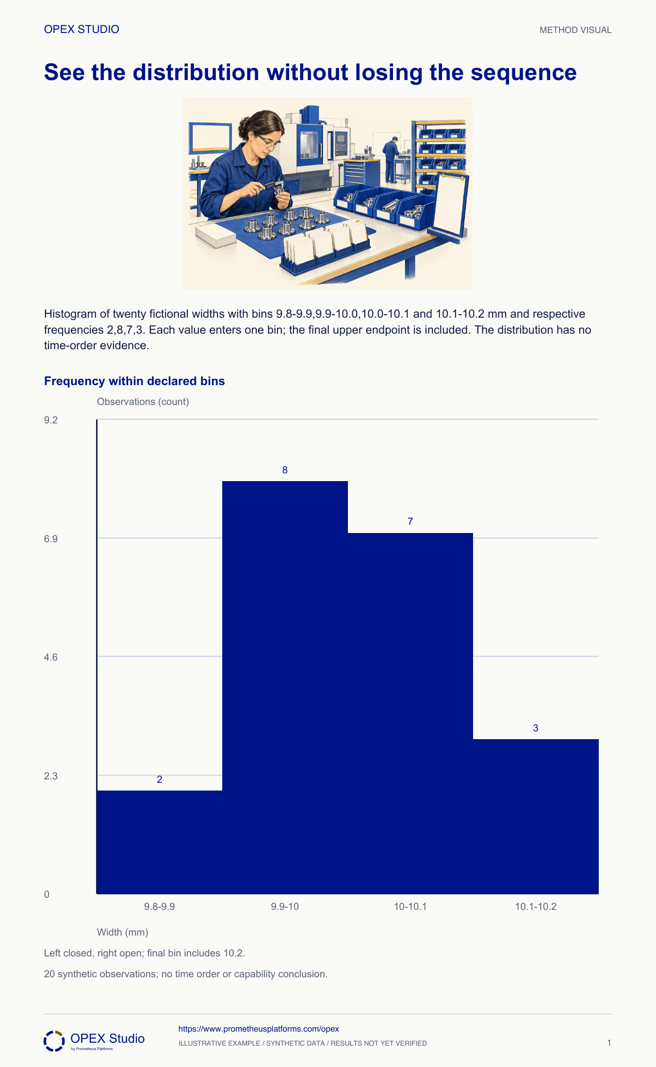
A histogram shows how observations occupy intervals of a measurement scale. Define contiguous bin edges and a rule for boundary values so every observation enters exactly one bin. Inspect shape, gaps and unusual values, while remembering that a histogram discards the sequence in which readings occurred. Two humps may suggest mixed sources, but they do not prove which sources are responsible. Keep the original time and source records for follow-up. A visually narrow distribution is also insufficient to establish stability or capability. Those conclusions require appropriate measurement evidence, temporal analysis and stated specification assumptions.
Bins 9.8–9.9,9.9–10.0,10.0–10.1,10.1–10.2 mm; counts 2,8,7,3.
Left-closed/right-open except final upper endpoint included.
Twenty synthetic points and no time order do not establish stability.
Fictional case: Alto Inspection groups twenty width measurements into bins from 9.80 to 10.20 mm. The core histogram retains counts 2, 8, 7 and 3. Analyst Nia must explain a width exactly equal to 10.00 mm and respond to a claim that the tidy shape proves the process is stable.
Keep the pooled distribution but prepare comparable source-separated views using the retained identities. Confirm measurement comparability and exposure before attributing differences.
A pooled shape can conceal different streams. A source label is useful evidence for investigation, not automatic proof that one machine caused the pattern.
Place measurements into explicit adjacent bins, reconcile the distribution, and preserve the time and source information needed for later questions.
Fictional case: Alto Inspection groups twenty width measurements into bins from 9.80 to 10.20 mm. The core histogram retains counts 2, 8, 7 and 3. Analyst Nia must explain a width exactly equal to 10.00 mm and respond to a claim that the tidy shape proves the process is stable.
Role: Quality analyst and measurement-record owner
Every measured value belongs to exactly one bin under a documented endpoint convention. Units, instrument resolution, observation identities and time order are retained.
Two spreadsheet users assign 10.00 to different bins; one includes it in both. The slide omits time order and calls the process controlled.
| Bin in mm | Count | Boundary convention |
|---|---|---|
| 9.80 to below 9.90 | 2 | Include 9.80; exclude 9.90 |
| 9.90 to below 10.00 | 8 | Include 9.90; exclude 10.00 |
| 10.00 to below 10.10 | 7 | Include 10.00; exclude 10.10 |
| 10.10 through 10.20 | 3 | Include both lower edge and final upper endpoint |
Nia names width in millimetres, the observation window and the twenty recorded units. She preserves the raw value and time for every observation before creating bins.
Why: A distribution removes sequence by design. Retaining the source records allows a later check for shifts, mixed streams or measurement issues without inventing missing data.
Evidence: Twenty identified measurements remain in the source table.
She uses left-closed/right-open intervals, with the final upper endpoint included. A reading of 10.00 therefore enters the third bin only.
Why: Adjacent bins require a convention at shared edges. The particular consistent convention is less important than preventing double counts or unassigned boundary values.
Evidence: The table explicitly defines the 10.00 and 10.20 assignments.
She sums 2 + 8 + 7 + 3 = 20 and compares that total with the raw observation count. She checks the units and equal bin widths before interpreting bar heights.
Why: Missing values or double-assigned boundaries can yield a plausible shape with a false total. Unequal-width histograms need a different height interpretation than this equal-width example.
Evidence: All twenty observations are accounted for once.
Nia says fifteen observations are in the middle two bins and identifies the observed range covered by the bins. She does not infer normality or stability from twenty grouped values.
Why: Grouping helps reveal distribution shape but hides ordering and individual detail. Several different time patterns can produce exactly the same histogram.
Evidence: The report describes this sample distribution with an explicit evidence limit.
To investigate stability, she retrieves the ordered measurements and operating context. To compare machines, she uses retained source labels rather than interpreting a pooled hump as a machine effect.
Why: The correct next view depends on the question. Repeated rebinning until the shape looks desirable would hide uncertainty instead of resolving it.
Evidence: Next analysis names time order or source grouping and the retained evidence it requires.
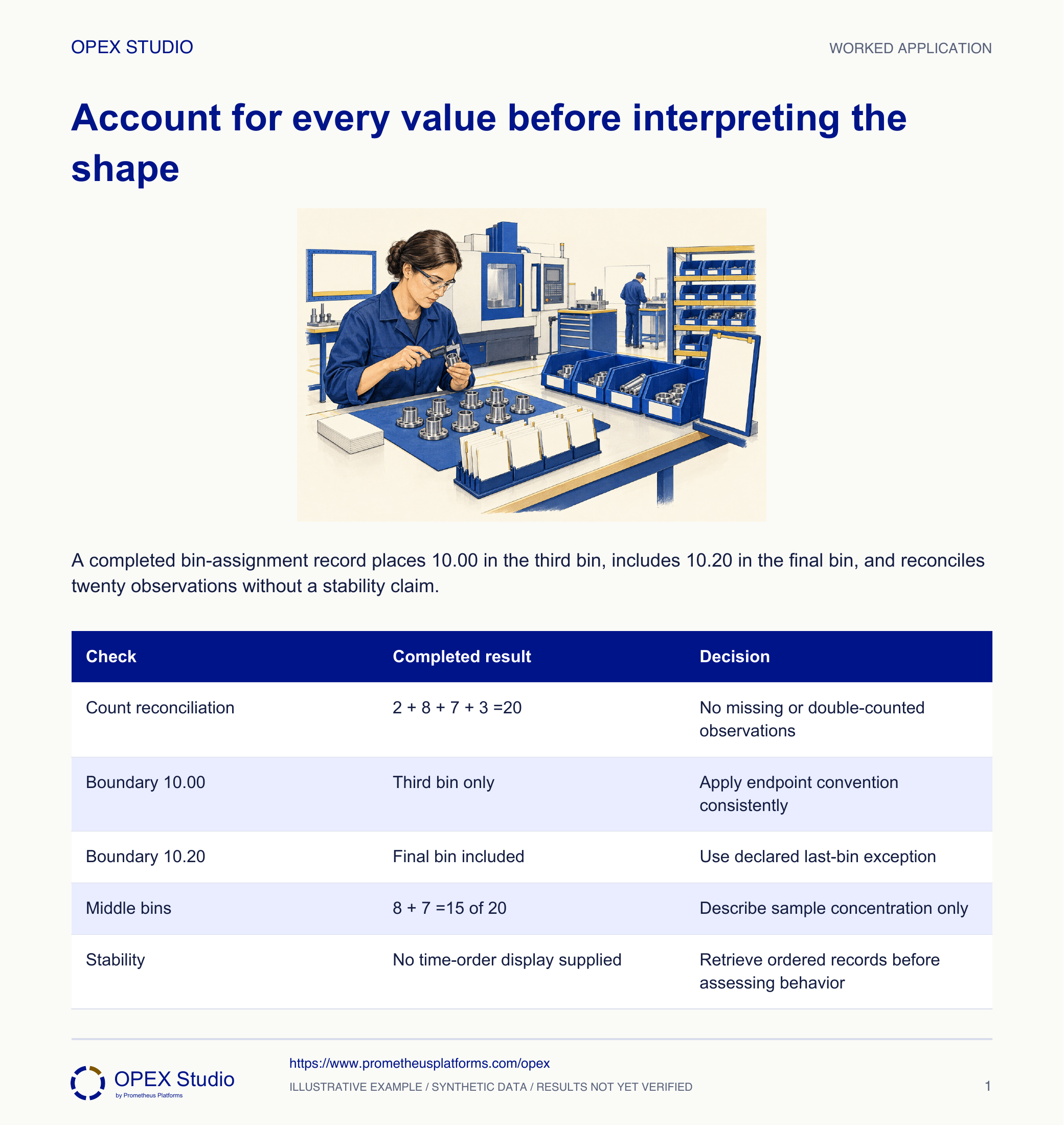
| Check | Completed result | Decision |
|---|---|---|
| Count reconciliation | 2 + 8 + 7 + 3 =20 | No missing or double-counted observations |
| Boundary 10.00 | Third bin only | Apply endpoint convention consistently |
| Boundary 10.20 | Final bin included | Use declared last-bin exception |
| Middle bins | 8 + 7 =15 of 20 | Describe sample concentration only |
| Stability | No time-order display supplied | Retrieve ordered records before assessing behavior |
The records reveal ten observations from each of two machines.
Keep the pooled distribution but prepare comparable source-separated views using the retained identities. Confirm measurement comparability and exposure before attributing differences.
A pooled shape can conceal different streams. A source label is useful evidence for investigation, not automatic proof that one machine caused the pattern.
The analyst can map each observation back to machine and time.
New fictional widths are 9.80,9.90,9.95,10.00,10.05,10.10,10.15 and 10.20 mm. Use the same four bins and endpoint convention.
| Bin | Learner task |
|---|---|
| [9.80,9.90) | Count values |
| [9.90,10.00) | Count values |
| [10.00,10.10) | Count values |
| [10.10,10.20] | Count values |
Counts are 1,2,2,3, totaling 8. The value 10.10 enters the fourth bin at its included lower edge;10.20 is included by the final-endpoint exception.
The same eight values could appear in rising order or alternate high/low. Those sequences have identical bin counts but different time behavior, so retain the original order and context.
| Bin | Assigned values | Count |
|---|---|---|
| First | 9.80 | 1 |
| Second | 9.90,9.95 | 2 |
| Third | 10.00,10.05 | 2 |
| Fourth | 10.10,10.15,10.20 | 3 |
Where should a shared-edge value go?
Try the convention before discussing shape.
Can the same values tell different time stories?
What information did grouping hide?
Place the eight numbers into bins on paper, then write a two-sentence interpretation and boundary.
Owner: Measurement-data owner
Record: Raw ordered values, bin rule and source-linked histogram
Review: At the next distribution review or any bin-rule change
Evidence: Reconciled counts and retained time/source identity
Correct collection or binning before comparing shapes; investigate ordering with an appropriate separate view.
A histogram displays the frequency distribution of numerical observations; bin choices and process context affect interpretation.
Public primary-source summary; underlying paid standards/forms are not reproduced.Read the lessons online or use these PDFs to prepare, practise and review with your team. No sign-in needed.
Case objectives, demonstration plans, debriefs, common mistakes and application checks across all 81 workplace cases and method lessons.
Download Facilitator guide PDF · 166 pages · 65.1 MBPrintable case worksheets, blank observation records and five calculation exercises; answers are separate.
Download Learner workbook PDF · 169 pages · 10.7 MBReasoned sample responses, worked calculations and coaching guidance; fictional examples are clearly labelled.
Download Answer key and coaching notes PDF · 105 pages · 8.5 MBThe native method mechanisms and worked applications for all 68 detailed lessons, in a separate bookmarked portrait reference.
Download Method and application reference PDF · 141 pages · 10.2 MBFive illustrated system chapters: 15 Flare concept maps and 26 original workplace teaching cards, with links to all 81 supporting cases and method lessons.
Download Illustrated systems atlas PDF · 69 pages · 55.8 MBExplore this connected method and its separate application conditions.
Explore the connected method →Explore this connected method and its separate application conditions.
Explore the connected method →Explore this connected method and its separate application conditions.
Explore the connected method →