Facilitator guide
Case objectives, demonstration plans, debriefs, common mistakes and application checks across all 81 workplace cases and method lessons.
Download Facilitator guide PDF · 166 pages · 65.1 MB OPEXSTUDIO
Define goal units/time. Follow the visual, practise a decision, then check your thinking.
Fictional teaching examples and AI-generated illustrations. Proposed changes and goals are not achieved results. Use the written instructions and check local conditions before applying a method.
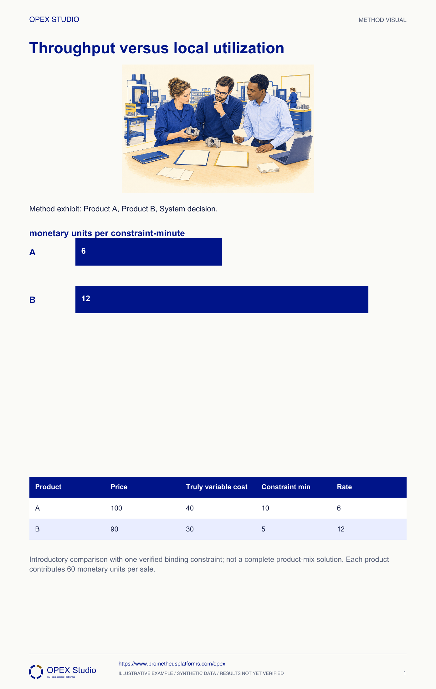
For a bounded decision, compare the effect on the system rather than local output alone. Financial throughput depends on sales and truly variable costs over a period; producing unsold stock does not create that throughput. In the single-constraint illustration, products A and B each provide 60 monetary units per sale, but use ten and five constraint-minutes respectively. Their rates are therefore six and twelve per constraint-minute. This helps frame a choice, but demand limits, other capacity, operating expenses and commitments still matter. Have finance validate definitions. Mission-led services should state their goal units instead of inventing a monetary proxy.
A: (100 − 40)/10 = 6 monetary units per constraint-minute; B: (90 − 30)/5 = 12.
The exercise assumes one binding constraint and comparable units. Demand, other capacity and commitments can change the decision.
Financial throughput requires sales; produced-but-unsold stock is not throughput. Finance must validate truly variable cost and expense definitions.
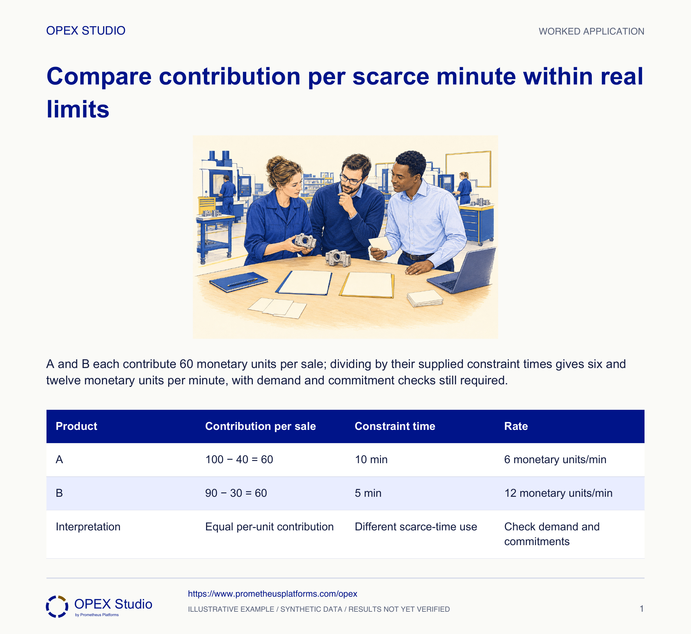
Fictional product comparison: A sells for 100 monetary units with 40 truly variable cost and consumes 10 minutes of the verified binding constraint. B sells for 90 with 30 truly variable cost and consumes five constraint-minutes. Analyst Noor compares the use of scarce time rather than rewarding every department for staying busy.
Do not make more B merely because its calculated rate is higher. Evaluate eligible A demand and the real remaining constraints.
The rate does not turn unwanted inventory into sold throughput.
Calculate throughput contribution per constraint-minute, apply demand and commitment limits, and distinguish the resulting teaching comparison from a complete profit or investment decision.
Fictional product comparison: A sells for 100 monetary units with 40 truly variable cost and consumes 10 minutes of the verified binding constraint. B sells for 90 with 30 truly variable cost and consumes five constraint-minutes. Analyst Noor compares the use of scarce time rather than rewarding every department for staying busy.
Role: Operations planner working with the accountable finance and commercial owners.
The selected feasible work supports sold throughput and commitments under the system’s real constraints.
Both products show a 60-unit contribution per sale, so the team assumes either mix uses the constraint equally well.
| Product | Price | Truly variable cost | Constraint time |
|---|---|---|---|
| A | 100 monetary units | 40 | 10 min/unit |
| B | 90 monetary units | 30 | 5 min/unit |
| Difference to calculate | Price minus truly variable cost | Per sold unit | Divide by constraint minutes |
Noor confirms the supplied truly variable cost is defined for the decision and sale, rather than an allocated share of unchanged overhead. She keeps operating-expense effects separate.
Why: A misleading cost basis can reverse the comparison. The teaching values are supplied, not a rule that every organization has only one kind of variable cost.
Evidence: A: 100 minus 40; B: 90 minus 30 monetary units per sale.
Both products contribute 60 monetary units before operating expense under the stated definition. Record the same result without assuming equal use of the constraint.
Why: Per-unit contribution describes a sale, not the rate at which limited capacity generates that contribution.
Evidence: A = 60; B = 60 monetary units per sold unit.
A uses ten minutes, yielding 60 / 10 = six monetary units per constraint-minute. B uses five, yielding 60 / 5 = 12.
Why: The denominator must be the verified limiting resource, not whichever machine is easiest to time.
Evidence: B has twice the supplied rate: 12 versus 6.
Use the rate to inform a feasible comparison only after checking how many units can be sold, which commitments must be met, and whether another resource or cost changes.
Why: Producing unsold B does not create the same goal outcome as selling it. A ranking alone is not a complete product-mix solution.
Evidence: Demand caps, minimum commitments and other constraints remain explicit decision inputs.
Review actual accepted sales, constraint use and relevant expense/investment consequences with the responsible owners. Do not claim profit from a local utilization increase.
Why: The rate is an introductory decision aid. Unchanged overhead, incremental expenses and real commitments still matter to the full decision.
Evidence: A documented feasible alternative and whole-system outcome replace an unsupported profit claim.
| Product | Contribution per sale | Constraint time | Rate |
|---|---|---|---|
| A | 100 − 40 = 60 | 10 min | 6 monetary units/min |
| B | 90 − 30 = 60 | 5 min | 12 monetary units/min |
| Interpretation | Equal per-unit contribution | Different scarce-time use | Check demand and commitments |
All currently sellable B demand is already covered. A still has confirmed demand.
Do not make more B merely because its calculated rate is higher. Evaluate eligible A demand and the real remaining constraints.
The rate does not turn unwanted inventory into sold throughput.
The decision records the B demand cap and the remaining feasible sales opportunity.
Separate fictional one-constraint exercise: C has price 120, truly variable cost 50 and 14 constraint-minutes per unit; D has price 105, cost 45 and six minutes. Available constraint time is 120 minutes. At least six C are committed; at most eight D can be sold. All units are indivisible and both products have sufficient eligible inputs.
| Input | Value |
|---|---|
| C | 120 − 50; 14 min/unit; minimum 6 units |
| D | 105 − 45; 6 min/unit; demand cap 8 |
| Constraint availability | 120 min |
| Model limits | One constraint; no additional expense effects supplied |
C contributes 70 per sale and 5 per constraint-minute. D contributes 60 and 10 per constraint-minute.
Six C consume 84 minutes, leaving 36; six D fit. This meets the C minimum and stays below the D cap.
The mix uses 120 minutes and contributes 6 × 70 + 6 × 60 = 780 monetary units before operating expense. Eight D would use 48 minutes and leave only 72, enough for five C, violating the six-C minimum.
| Allocation | Constraint use | Contribution / conclusion |
|---|---|---|
| C | 6 × 14 = 84 min | 6 × 70 = 420 |
| D | 6 × 6 = 36 min | 6 × 60 = 360 |
| Feasible total | 120 min | 780 before operating expense |
| Eight-D-first | Only 5 C fit | Minimum commitment violated |
Which costs and scarce time are actually supplied?
Why does equal contribution not imply equal rate?
How does the commitment change a rate-only preference?
What is missing before anyone can call this profit?
Calculate each rate, write constraints separately, then audit the feasible quantities before checking the solution.
Owner: System/planning owner with finance and commercial authority
Record: Decision assumptions, feasible mix comparison and observed sold outcome
Review: Before committing a real mix and after material demand/capacity/cost changes
Evidence: Accepted sales, relevant expense effects and constraint/commitment compliance
Rebuild the comparison when constraints or assumptions change; obtain the missing decision data.
Totally variable cost definition
Method reference; original OPEX scenario and diagram are synthetic teaching content, not source case results.Throughput is rate of goal units; sold rather than merely produced units; global T/I/OE measures. Historical terminology source.
Method reference; original OPEX scenario and diagram are synthetic teaching content, not source case results.Read the lessons online or use these PDFs to prepare, practise and review with your team. No sign-in needed.
Case objectives, demonstration plans, debriefs, common mistakes and application checks across all 81 workplace cases and method lessons.
Download Facilitator guide PDF · 166 pages · 65.1 MBPrintable case worksheets, blank observation records and five calculation exercises; answers are separate.
Download Learner workbook PDF · 169 pages · 10.7 MBReasoned sample responses, worked calculations and coaching guidance; fictional examples are clearly labelled.
Download Answer key and coaching notes PDF · 105 pages · 8.5 MBThe native method mechanisms and worked applications for all 68 detailed lessons, in a separate bookmarked portrait reference.
Download Method and application reference PDF · 141 pages · 10.2 MBFive illustrated system chapters: 15 Flare concept maps and 26 original workplace teaching cards, with links to all 81 supporting cases and method lessons.
Download Illustrated systems atlas PDF · 69 pages · 55.8 MBExplore this connected method and its separate application conditions.
Explore the connected method →Explore this connected method and its separate application conditions.
Explore the connected method →Explore this connected method and its separate application conditions.
Explore the connected method →